Domain adaptation is an important area in transfer learning. The goal is grand: to deploy a model on a different domain from which it was trained on. A domain can be simply thought of as a different class of data. One of the examples is sentiment analysis on customer reviews of different types of products. Imagine that we have trained a sentiment classifier of books and were given a number of unlabeled data on DVD, how should we adapt this classifier to DVDs? Can we stretch the classifier to kitchen appliances?
On the one hand, each domain has their unique determining features. For example, ‘boring’ is a strong indicator of a negative review for a book but we rarely use it to describe a knife. On the other hand, the two domains are related; e.g., ‘great’ can be used for both. The question is how to adapt the model trained on one domain to another. This blog is on the instance-weighting methods and feature enhancement will be introduced in the coming one.
Related literature
An excellent introduction to the framework of transfer learning used in classification and regression tasks is Pan and Yang (2009) and a more recent survey is Weiss et al. (2016). The other field of application of transfer learning is reinforcement learning.
In this blog, the instance-weighting method for domain adaptation will be explored. The work is base on the PhD thesis of Jing Jiang (2008). A topic that is related is covariance shift and sample selection bias.
Algorithms
Problem definition
We have lots of labeled data in one domain, called source domain, and we hope to make predictions in another domain, named target domain, where we have many unlabeled data. One scenario is that there is no labeled data in the target domain, often known as an unsupervised algorithm. The other possibility is to have a small number of labeled data, i.e., semi-supervised learning.
Notations
- Input from feature space $\mathcal{X}$
- Output to the label space $\mathcal{Y}$
- Source domain $\mathcal{D}_s$ :
- With $N_s$ labled data points ${(x^s_1, y^s_1), …, (x^s_{N_s}, y^s_{N_s}) }$
- Target domain $\mathcal{D}_t$ :
- With $N_{t,l}$ labled data points ${(x^t_1, y^t_1), …, (x^t_{N_{t,l}}, y^t_{N_{t,l}}) }$
- With $N_{t,u}$ unlabled data points ${x^t_1, …, x^t_{N_{t,u}}}$
- Ensemble of input $X$ an output $Y$
- Hypothesis space: $\mathcal{H}$
- Model $f$: in this case the model is a classifier.
A probabilitistic framework
Emprical risk minimisation
A general machine learning framework is to find the optimal model $f^*$ from candidate models from the a hypothesis space $f \in \mathcal{H}$ that minimises the the cost function $L(x,y,f)$. It can be formulated as:
Domain adaptation
To find the optimal model for the target domain with only source domain data, we rewrite the above equation as such
For discrete data ${(x^s_1, y^s_1), …, (x^s_{N_s}, y^s_{N_s}) }$:
Expanding using the product rule:
In summary, there are two types of differences:
- Instance difference: $P_t(Y\vert X) = P_s(Y\vert X)$ but $P_t(X) \neq P_s(X)$.
- The dependency of the label on the data are the same but the density of feature space are different.
- Same problem as covariance shift or sample selection bias.
- Labeling difference: $P_t(Y\vert X) \neq P_s(Y\vert X)$ .
- The dependency of the label on the features are different.
Say we are doing domain adaptation for British people and given non-British sample. For example, the probability of British and non-British people to talk about the weather is the same given it rains $P_t(Y\vert X) = P_s(Y\vert X)$ but the probability of raining is different $P_t(X) > P_s(X)$. Thus British people are more likely to talk about the weather. For the second scenario, the extent of positiveness is much less for British people when they use the word ‘interesting’, i.e., $P_t(\text{positive}\vert \text{interesting})< P_s(\text{positive}\vert \text{interesting})$ , which might make our sentiment classifier to fail.
The two difference are noted as $\alpha_i$ and $\beta_i$ an we then discuss how to estimate $\alpha_i$ and $\beta_i$.
Estimating $\alpha_i$
$\alpha_i$-weighting can be used in both unsupervised and supervised learning framework. We can train a model to predict the marginal probabilities $P_s(X)$ and $P_t(X)$, where $P_t(X) = 1- P_s(X)$. A straight-forward framework to use is the logistic classifier. In a regularised framework for unsupervised learning:
where $\alpha_i = \frac{P_t(x^s_i)}{P_s(x^s_i)}$ and assume $\beta_i = 1$. $\lambda$ is the regularisation parameter for the regulariser $R(f)$.
Estimating $\beta_i$
We will discuss the estimation of $\beta_i$ under the supervised learning framework, i.e., given a small number of labeled target data. The optimisation problem needs updating:
where $\lambda_s, \lambda_{t,l}$ are trade-off parameters that balances the two populations. Note that we drop the $\frac{1}{N_s}$ term but require that $\sum_{i=1}^{N_s} \alpha_i\beta_i = N_s$.
By training the models to predict $P_s(Y\vert X)$ and $P_t(Y\vert X)$ using the labeled source domian and target domain data, we can substitute $\beta_i$ using the definition $\frac{P_t(y^s_i \vert x^s_i)}{P_s(y^s_i \vert x^s_i)}$.
Heuristic: upweight labeled target data
Jiang (2008) also proposed a method to upweight the labeled domain data such that of the small number of labeled target samples has the same weight as the large number of labeled source data, i.e., set $\lambda_{t,l} = \lambda_s \frac{N_{s}}{N_{t,l}}$. It was also recommended to use even higher $\lambda_{t,l}$.
Experiments and Results
We tested the methods in the instance-weighting framework using two datasets:
- The ECML KPDD 2006 challenge for spam classification: labeled source data 4000, unlabeled target data 2500.
- The amazon sentiment analysis dataset from Blitzer et al. (ACL 2007) using labeled source data 2000 and target data 2000.
The results are in the two notebooks: Spam: instance weighting and Sentiment: instance weighting.
The accuracy of $\alpha$-weighting decreases for both examples.
The accuracy of supervised learning using different sample sizes are summarised in the two figures blow. In the sentiment analysis task, we show the results for domain adaptation from DVD to Kitchen.
The five models are
- BL: baseline with source data only
- Beta: $\beta$-weighting using a model trained on the labeled target data: $\beta = \frac{P_t(y^s_i \vert x^s_i)}{P_s(y^s_i \vert x^s_i)}$
- BL+LT: baseline with source + labeled target data
- LT+beta: source + labeled target data + $\beta$-weighting
- Upweighted LT: source + upweighted labeled target data
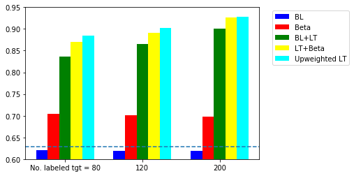
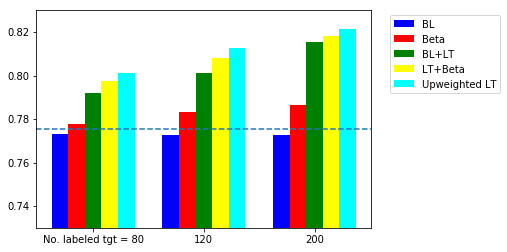
Comparing the scenarios with and without $\beta$-weighting, there is improvement by including $\beta$-weighting. It means that the classification task is the domain-specific. For example, if mentioning money or transcation is a key indicator for spam email, it may not be the case for a person working in finance. The up-weighting performs better than using $\beta$-weighting. The take-away message is the significance of labeling a small number of target domain.
Details of implementation
All the details are in the Jupyter notebooks and some key points are listed below.
Data pre-processing
- The raw inputs were word counts (no specific word is given in the spam data). We converted it into a matrix, where each column represent the counts of a certain word.
- The most frequent 10,000 words were selected as features.
Base case
- Logistic regression: the prediction is in sensitive to the regularisation parameter and are thus set to 1.
Supervised learning
- All classification models used logistic regression (C = 1)
- Labeled target data were chosen randomly.
- 8 different labeled/unlabeled splits were tested.
Future work:
- Two $\alpha$-weighting methods were proposed in the thesis.
- First one is the same in nature with logistic regression but the exact optimisation formulation was not reproduced.
- The second is called mean matching that minimises the distance between the mean of the target and source domain. I attempted it but need to upgrade my optimisation skills.
- The insight into how to measure the difference between two domains is needed. One promising direction is the four types of difference discussed Jiang (2008).
- Features that are frequent in source domain but infrequent in target domain
- Features that are infrequent in source domain but frequent in target domain
- Features that are discriminative in source domain but non-discriminative in target domain
- Features that are non-discriminative in source domain but discriminative in target domain
- Semi-supervised learning or ‘bootstrapping’ was also proposed. In this case, the unlabeled data are treated as source data and are used to train the classifier.