After introducing the instance weighting framework for domain adaptation in the previous blog, I will explore a different framework. The second category of algorithms is feature-based. Instead of taking each instance as a whole, we try to extract useful information from the features. Here we explore three algorithms and applied them on the sentiment analysis adaptation.
- Frustratingly easy domain adaptation (FEDA) by Daume (2007): Juypter notebook
- Structural correspondence learning (SCL) by Blitzer et al. (2006): Jupyter notebook
- Spectral Feature Alignment (SFA) by Pan et al. (2010) : Notebook to replicate the original paper, a simplified agile version
All three algorithms seek to augment the features and seek how the two domains overlap. Regarding the features, there are three types of differences between domains
- The marginal probabilities (i.e., $P(X)$) for the features are different but their relationship with the outcome (i.e., conditional probability $P(Y\vert X)$) are the same . E.g. ‘great’, ‘worst’ are generic comments for different product types.
- The feature is present in one domain but absent in the other. E.g. we use ‘boring’ to comment on a movie but hardly use it to describe a knife.
- The feature has opposite meanings in two domains, i.e., $P(Y\vert X)$ are different. E.g. ‘small’ is positive for a smartphone but negative for a hotel room.
*Ongoing notes on transfer learning and the algorithms can be found here.
Frustratingly easy domain adaptation (FEDA)
FEDA applies to supervised learning setting. Daume (2007) introduces an augmented feature space defined by the following mapping functions ($\vec{0}$ has the same length as $\vec{x}$):
- For source domain: $\vec{\Phi}^s = \langle \vec{x},\vec{x},\vec{0} \rangle$
- For target domain: $\vec{\Phi}^t = \langle \vec{x},\vec{0} ,\vec{x}\rangle$
All vectors are of the same length such that each feature, e.g. the word ‘good’, will be duplicated three times: (1) shared feature space (2) source feature space and (3) target feature space. Then the classification will be trained on the augmented feature space, e,g, using logistic regression.
To gain some insight, let us consider the possible outcomes of the classifier weights of three features for smartphone (source) and hotel (target) domains. Empty cells shows independency; ‘+’ weight contributes to positive sentiment and ‘-‘ for negative sentiment.
| Features | good | small | parking | good | small | parking | good | small | parking |
|---|---|---|---|---|---|---|---|---|---|
| Smartphone | + | 0 | 0 | 0 | + | 0 | |||
| Hotel | + | 0 | 0 | 0 | - | + |
- ‘good’ is a shared feature for positive sentiment so that it has positive weight in the shared feature space.
- ‘small’ has opposite meaning in the two domains so that it has positive weight in the smartphone feature space but negative weight in the hotel feature space.
- ‘parking’ is only present in the hotel domain so its weight is captured in the target feature space.
We can see that FEDA can address all three types of differences. Regarding the difference in marginal distribution (type 1), say ‘interesting’ occurs more frequently in smartphone than hotel reviews, the weights can be distributed between the joint space and the source (smartphone) feature space.
There is a neat kernelised interpretation for this. In the simplest form: $\vec{\Phi}^s \vec{\Phi}^s = 2\langle x,x’\rangle$ and $\vec{\Phi}^s \vec{\Phi}^t = \langle x,x’\rangle$. The advantages of FEDA are simple implementation and interpretability. However, when the two domains are similar, Weiss et al. (2016) commented that FEDA tends to underperform.
Test results
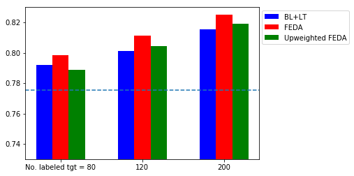
First, FEDA yields more accurate prediction than the baseline trained on both the source and target domain, suggesting that it captures the difference between domains. Compared with the instance weighting results, FEDA is comparable to the $\beta$-weighting and upweighted scenarios.
Besides FEDA, I also tried an upweighted implementation, where the labeled domain is assigned the same weight as the unlabeled target domain. However, it does not perform as good as FEDA. One possible reason is that when the number of labeled target data is too small (80), the high weight (25 times higher than the source data) forces the classifier to overfit to the labeled target data. As we can see, the upweight is slightly better than the baseline when more labeled target data is available. The weight of labeled target data was suggested by Daume (2007) to be incorporated as a hyperparameter.
Interpretability
The second part of the notebook explores the interpretability using $\ell_1$-penalty to promote the sparsity. $\ell_1$-penalty forces the weights to be sparse, meaning that only weights of important features are nonzero. Here are some insight
| Domain | positive | negative |
|---|---|---|
| shared features | love, going strong, great | disappointment, worst, horrible, waste |
| DVD source domain | bonus, classic, gem | lame, boring, dull |
| kitchen target domain | nice, stars, easy, durable | broken, returning, thermometer |
Structural correspondence learning (SCL)
The underlying reasoning of SCL is to find correspondence of features from the source domain to the target domain. This is done via shared features called ‘pivot features’ in SCL. For example,
- Kitchen review: An absolutely great purchase…This blender is incredibly sturdy
- DVD review: A great moview … It is really a classic.
Great is a pivot feature while sturdy and classic correspond to each other in the two domains. Below is a map of corresponding features in the ICML tutorial slide for book and kitchen reviews.
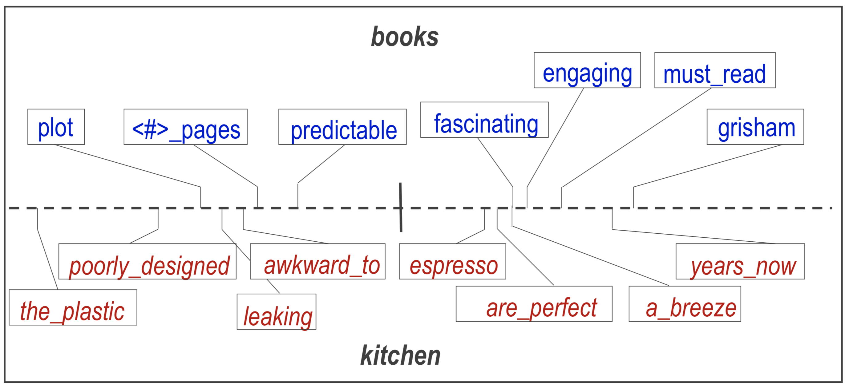
We will never use ‘the plastic’ to desribe a book but it if we know it correspond to ‘plot’ in book domain, we are likely to have more reliable features, thus increasing the accuracy of prediction. SCL incorporate this corresponce as an enhanced feature space.
Algorithm
The algorithm is the following
- Define pivot features.
- Train pivot predictors to find the correspondence of features with pivot features.
- Use SVD to find low-dimensional feature mapping.
- Use low-dimensional feature mapping to enhance the original feature.
Step 1: pivot feature selection
Blitzer et al. (2006) used the most frequent features as pivot features; Blitzer et al. (2007) showed that using the features with high mutual information, i.e., with higher correlation with the label/prediction, improves the final outcome.
Step 2: Pivot predictors
Given $l$ pivot features, train $m$ linear predictors on all the data.
The weight vectors $\hat{\vec{w}}$ encode the covariance of the non-pivot features with the pivot features. Using the vectors, we can build a matrix
Step 3: Low-dimensional feature mapping
From the SVD of $W$ given by $W= U\Sigma V^T$, we can construct a low-dimensional feature representation $\theta$ using the first $h$ left eigenvector, i.e.
Step 4: Enhanced feature space
The low-dimensional feature space is $\theta^T \vec{x}$, thus the enhanced feature space is $[\vec{x}, \theta^T \vec{x}]$. We train the classifier using ${[\vec{x^s_i}, \theta^T \vec{x^s_i}], y^s_i}$ then make predictions using ${[\vec{x^t_i}, \theta^T \vec{x^t_i}]}$
Test results
In comparison to FEDA, SCL is an unsupervised learning algortihm. By tuning the regularisation parameter in a train/development split of 9/1, the accuracy increased from 0.774 to 0.801. SCL is also interpretable by examining the weights of the singular vectors.
| Singular vector | positive | negative |
|---|---|---|
| 1st | great, very, easy, good | waste, money, worst, worst of |
| 2nd | best, a great, the best, love | waste, boring, terrible |
| 3rd | best, well, excellent | great, waste, terrible |
One interesting thing is the ‘mixed’ sentiment from the third singular vector, suggesting that the underlying low-dimensional space may be only 2D. Also the words that have highest weight also coincide with the pivot features.
Some other interesting tests I tried are
- Using only the low-dimensional subspace ($\theta^T \vec{x}$) instead of the enhanced feature space $[\vec{x}, \theta^T \vec{x}]$
- Same accuracy as enhanced feature space
- Trying to weight the low-dimensional subspace differently $[\vec{x}, \text{weight}\times\theta^T \vec{x}]$ .
- Improvement given weight from 1 to 5.
- Insensitive to the enhancement for weight > 5
- Excluding pivot features when building the low-dimensional subspace.
- Slightly underperformed (0.795)
Spectral Feature Alignment (SFA)
SFA is very similar to SCL; SFA provides a different way to compute the low-dimensional feature space. The pivot features are domain independent features that are common in both domains. SFA finds a mapping from domain specific features to domain independent features using the graph spectral theory.
Immitating Pan et al (2007) Fig. 1, we use a simple example to demonstrate the core idea.
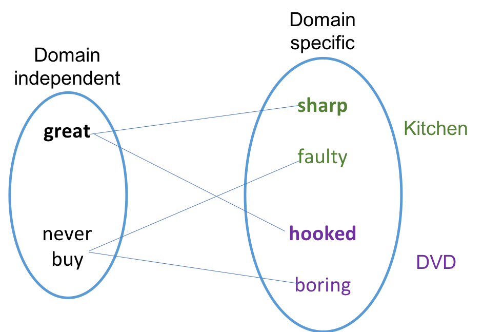
Imagine we have only 4 examples, the co-occurence matrix of domain specific and domain independen words
| sharp | hooked | faulty | boring | |
|---|---|---|---|---|
| great | 1 | 1 | 0 | 0 |
| never buy | 0 | 0 | 1 | 1 |
Following the algorithm, we find that the two vectors for low-dimensional mapping are $[0.5,0.5,0,0]$ and $[0,0,0.5,0.5]$. The two vectors maps the feature ‘sharp’ and ‘hooked’ from the two domains onto the same dimension and ‘faulty’ and ‘boring’ onto the same dimension.
To summarise, SCL and SFA can both solve difference types 1 & 2 but fails to distinguish the features that have opposite meaning in the two domains.
Test result
However, I failed to replicate the original results from Pan et al. (2010). Later attempt was made to create a simple toy example using two meaningful domain independent features (great and waste) and using only 100 features. The accuracy was 0.824 for the base case while improves only to 0.834 given after tuning the trade-off parameter $\gamma$.
Future work
- Kernelised version for FEDA: to improve understanding of kernel and what are the potential benefits of kernels.
- SCL: combine supervised learning as in Blitzer et al. (2007); how to select the best number of features and determine the dimension of projection.
- SFA: investigate the failure fore replicating the original work.
Appendix
FEDA table discussion
In the table, the weights ‘0’ may not be negligible If ‘good’ is a common feature for positive sentiment, it will contribute to all three copies of the same feature. Using $\ell_1$-penalty may improve this situation but when I tested $\ell_1$-penalty, the accuracy drops slightly. I guess having more weights on the duplicates is beneficial, similar to the increased accuracy with upweighted low-dimensional feature space in ‘SCL’.
SFA algorithm
Step 1: Find domain-independent features
Separate $m$ features into $l$ domain-independent features $W_{DI}$ and $m-l$ domain-specific features $W_{DS}$.
Step 2: Construct the co-occurence matrix M
For any element in matrix $\textbf{M}$, $m_{ij}$ is the total number of co-occurrence of $w_i \in W_{DS}$ and $w_j \in W_{DI}$ in both source and target domain. Given two binary matrices showing the occurence of feature $W_{DI}$ and $W_{DS}$ in each example (a total of $N = N_s + N_t$).
The weight matrix is
Step 3: Spectral feature clustering
- Form a weight matrix $\textbf{M}$
- Form an affinity matrix $\textbf{A} = \left[ \begin{array}{cc} \textbf{0} & \textbf{M} \ \textbf{M}^T & \textbf{0} \end{array} \right]$
- Form a diagonal matrix $\textbf{D}$ where $D_{ii} = \sum_j \textbf{A}_{ij}$ and construct the matrix $\textbf{L} = \textbf{D}^{-1/2}\textbf{A}\textbf{D}^{-1/2}$
- Find the $K$ largest eigenvectors of $\textbf{L}$ and form the matrix $\textbf{U}$
- Define feature mapping function $\varphi(x) = x\textbf{U}_{[1:m-l, :]}$
Step 4: Feature augmentation
Enhance each data with the feature mapping function, whose input are the domain specific features. There is a trade-off parameter $\gamma$ that balances the two spaces.